Markov chains and chaos

In my previous post, we explored the dyadic transformation $x_{n+1}=2x_n\bmod1$ on [0,1). We found its behavior was dependent on whether $x_0$ was rational or irrational. We also found if we repeatedly applyed the map to an initial set of particles, its density converged towards the uniform density.

$$ x_{n+1} = \begin{cases} x_n + 2^\alpha x_n^{1+\alpha} & 0\le x_n<1/2 \\ 2x_n - 1 & 1/2\le x_n<1 \end{cases} $$

where $\alpha\in[0,1]$ is some parameter controlling the concavity. Herein we refer to this map as the $\alpha$-map.

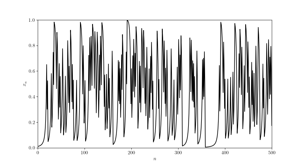
Looking at an individual orbit of the $\alpha$-map (with $\alpha=0.6$), we see the $\alpha$-map appears to preserve the chaotic nature of the dyadic transformation.

Unfortunately, proving that is chaotic is not as simple as before. It is also not as simple to determine its invariant density. With the dyadic transformation we made use of transfer operators.

Definition.¹ Let $f:M\rightarrow M$ be a surjective map such that the preimage $f^{-1}(x)$ is finite or countable for each $x\in M$. The Ruelle transfer operator $\mathcal{L}_f:\mathcal{F}(M,\mathbb{C})\rightarrow\mathcal{F}(M,\mathbb{C})$, where $\mathcal{F}(M,\mathbb{C})$ is the vector space of functions from $M$ to $\mathbb{C}$, is the linear operator given by

$$ (\mathcal{L}_f\varphi)(x) = \sum_{y\in f^{-1}(x)}\frac{\varphi(y)}{|\det Df(y)|}. $$

Some sources replace the Jacobian determinant with a more general function $g$ with the constraint that $\sum_{y\in f^{-1}(x)}g(y)$ converges for all $x$.

Once you’ve computed the transfer operator of a map, its corresponding invariant density would be given by finding the eigenfunction corresponding to the eigenvalue 1.

For example, if we generalize the dyadic transformation to the form

$$ x_{n+1} = rx_n\bmod1 $$

for some positive integer $r$, then we can find the induced transfer operator is of the form

$$ (\mathcal{L}_r\rho)(x) = \frac{1}{r}\sum_{k=0}^{r-1}\rho\left(\frac{x+k}{r}\right). $$

From here it is clear that the uniform density $\rho(x)=1$ is the invariant density since $\mathcal{L}\rho=\rho$.

However, if we try to find the transfer operator for the $\alpha$-map we reach a dilemma. While inverting $x_{n+1}=2x_n-1$ is trivial, finding the inverse of $x_{n+1}=x_n+2^\alpha x_n^{1+\alpha}$ is not. We need a different technique.

Enter Markov chains! If we partition our space [0,1) into a finite set of intervals $I_1,\dots,I_n$, then we can use Markov chains to approximate the invariant density. Namely, we use the transition matrix $P$ where $p_{ij}$ is the probability that if $x\in I_i$ then $f(x)\in I_j$. This we can compute with the image, i.e.,

$$ p_{ij} = \frac{m(f(I_i)\cap I_j)}{m(f(I_i))}, $$

where $m$ is the Lebesgue measure. Lets test this on our dyadic transformation. If we partition [0,1) into [0,1/2) and [1/2,1) we get the following Markov chain:

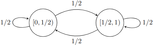
If you remember Markov chains, to find the invariant distribution we find the left eigenvector of the transition matrix corresponding to the eigenvalue 1, i.e., the vector $\pi$ such that $\pi P=\pi$. The transition matrix for the Markov chain above is given by

$$ P = \frac{1}{2}\begin{bmatrix} 1 & 1\\ 1 & 1 \end{bmatrix}. $$

and $(1/2,1/2)P = (1/2,1/2)$. Converting this back to density functions we get that the dyadic transformation has an invariant density of

$$ \rho(x) \approx \frac{\pi_i}{m(I_i)}, x\in I_i, $$

which for the dyadic transformation gives us $\rho(x)\approx 1$, the exact solution.

With this method, we can approximate the invariant density for the $\alpha$-map as finding the image is much easier than the preimage. The first question is how to form our partition? Through numerical simulations we found that the invariant density appears to be propotional to $x^{-\beta}$ for some unknown contant $\beta$. This result makes sense. If you look at the flow of the $\alpha$-map, we find it’s smallest near zero. Therefore, we expect particles to cluster around zero.

So our partition should have smaller bins near zero and larger bins near one. One way to accomplish this is to take the partition $P_n={0=b_0<b_1<\cdots<b_k=1}$ where $b_i=\left(\frac{i}{k}\right)^n$. Then as $n$ increases we should get better approximations. If we then approximate the exponent $\beta$, we get the data below:

$\alpha$	$P_4$	$P_5$	$P_6$	$P_7$	$P_8$
0.2	-0.1687	-0.1808	-0.1883	-0.1943	-0.1965
0.4	-0.3886	-0.3959	-0.3985	-0.3995	-0.3998
0.6	-0.5972	-0.5994	-0.5999	-0.5999	-0.5999
0.8	-0.7994	-0.7999	-0.7999	-0.7999	-0.8

Notice that the exponent $\beta$ appears to converge to $-\alpha$ as $n$ grows larger.

Conjecture. The $\alpha$-map has an invariant density of $\rho(x)=(1-\alpha)x^{-\alpha}$.

References Link to heading