In Nonlinear Dynamics and Chaos by Steven Strogatz, the following definition of chaos is given:
Chaos is aperiodic long-term behavior in a deterministic system that exhibits sensitive dependence on initial conditions. (Strogatz, p. 331)
The Dyadic Transformation Link to heading
On $[0,1)$ define the recurrence relation
$$ x_{n+1} = 2x_n\bmod1 = \begin{cases} 2x_n & x_n < 1/2 \\ 2x_n-1 & x_n \ge 1/2 \end{cases}. $$The above relation forms a discrete dynamical system on the space $[0,1)$. Consider the following graph of an orbit.
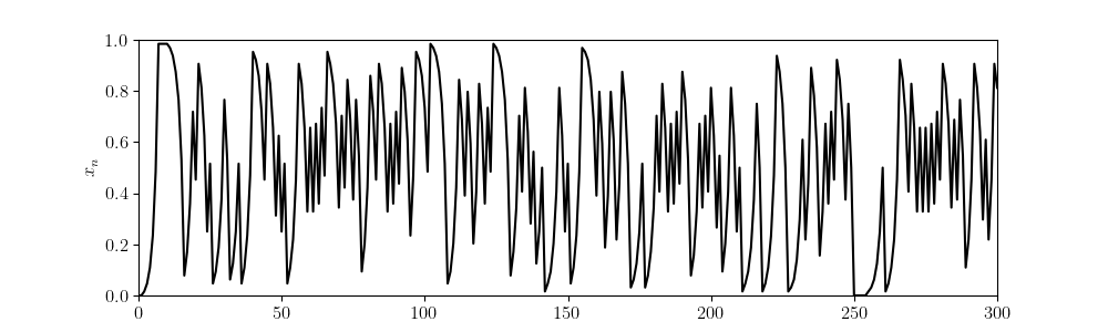
The orbit appears chaotic. However, as we will see later whether ${x_n}$ is periodic depends on our initial condition $x_1$.
It is worth noting some computation issues with this system. Consider the number 0.15625 in float32:

Therefore, $x_n$ will converge to 0. We can see this in action in the table below.
We could avoid this problem by using different bases in our representation. However, this still doesn’t capture the chaotic behavior. For example, consider the orbit starting at 1/5:
$$\frac{1}{5}\rightarrow\frac{2}{5}\rightarrow\frac{4}{5}\rightarrow\frac{3}{5}\rightarrow\frac{1}{5}.$$The sequence starting at 1/5 is periodic with period 4.
Thereom. If $x_1$ is rational, then ${x_n}$ converges or is eventually periodic.
$$ x_{n+1} = 2\left(\frac{a_n}{b}\right)\bmod 1 = \frac{2a_n\bmod b}{b}. $$So the set of possible values for $x_{n+1}$ is ${0/b,1/b,\dots,(b-1)/b}$ which is finite. Therefore, $x_n=x_{n+p}$ for some $p\in\mathbb{N}$. $\Box$
If our system does actually exhibit chaos, then it must be with an irrational number. While we can’t use floats to represent irrational numbers, there are other tricks we can use. Our system turns out to work nicely if the term is expressed in binary since multiplying by 2 is equivalent to bit shifting one to the left.
$$2x\bmod1 = (0.a_2a_3a_4\cdots)_2.$$The orbit graph above was formed by taking a random sequence of 0’s and 1’s then repeatedly removing the first element of the sequence and plotting the approximate value.
Theorem. If $x_1$ is irrational, then ${x_n}$ is aperiodic.
$$ x_n = (0.a_na_{n+1}a_{n+2}a_{n+3}\cdots)_2.$$Since $x_1$ is irrational, the digits $a_1,a_2,\dots$ have no repetition. Therefore, ${x_n}$ is aperiodic. $\Box$
Distribution Dynamics Link to heading
Assume we have a subset $X\subset[0,1)$ with some probability density $\rho_1(x)$. In other words, the probability that some $x\in A\subset X$ is given by
$$\mathbb{P}(x\in A) = \int_A \rho_1(x)\textup{d}{x}.$$We are interested in how the distribution changes over time. More precisely, let $\rho_2$ be the probability density of the image $(2x\bmod1)(X)$. Repeating this, forms a sequence of probability density functions ${\rho_n}$.
We want to find a linear operator $\mathcal{L}$ such that for any density $\rho_n$, $\rho_{n+1}=\mathcal{L}\rho_n$. If such an operator exists, then
$$\mathbb{P}(x_{n+1}\in A) = \mathbb{P}(x_n\in(2x\bmod1)^{-1}(A)).$$So
$$ \int_A\mathcal{L}\rho(x)\textup{d}x = \int_{(2x\bmod1)^{-1}(A)}\rho(x)\textup{d}x.$$To determine the operator $\mathcal{L}$, let $A=[0,y]$ for some $y\in[0,1)$. Note that $2x\bmod 1$ is two-to-one, and we can explicity determine the preimage. That is,
$$(2x\bmod1)^{-1}([0,y]) = \left[0,\frac{y}{2}\right]\cup\left[\frac{1}{2},\frac{y+1}{2}\right].$$$$ \begin{align*} \int_0^y\mathcal{L}\rho(x)\textup{d}x &= \int_{(2x\bmod1)^{-1}([0,y])}\rho(x)\textup{d}x \\ &= \int_0^{y/2}\rho(x)\textup{d}x + \int_{1/2}^{\frac{y+1}{2}}\rho(x)\textup{d}x. \end{align*} $$Differentiating both sides gives
$$ \mathcal{L}\rho(x) = \frac{1}{2}\rho\left(\frac{x}{2}\right) + \frac{1}{2}\rho\left(\frac{x+1}{2}\right).$$Remark. The linear operator $\mathcal{L}$ is a Ruelle transfer operator.
With our operator $\mathcal{L}$, we get the sequence of density functions $\rho_n=\mathcal{L}^n\rho_1$. Consider the limit
$$\lim_{n\rightarrow\infty}\mathcal{L}^n\rho_1=\rho_\infty.$$If the limit exists, then $\mathcal{L}\rho_\infty=\rho_\infty$. That is $\rho_\infty$ is the invariant density under $\mathcal{L}$. Notice that if $\rho(x)=1$, then
$$\mathcal{L}\rho(x) = \frac{1}{2}\rho\left(\frac{x}{2}\right) + \frac{1}{2}\rho\left(\frac{x+1}{2}\right) = 1.$$Therefore, the uniform density $\rho(x)=1$ is the invariant density under $\mathcal{L}$.
This tells us that for any initial density of particles, repeatedly applying $2x\bmod1$ results in the particles spreading out to the uniform density.